Personalized Pagerank for link prediction

I read Edwin Chen`s blog(who is famous data scientist, my role model!) and read interesting post.

Problem was Edge Prediction in given social graph. after I read through Edwin`s blog, I decided to implement it with Map/Reduce since I am not fluent with Scalding and scalar yet(These days I have been busy to catching up Functional Programming course from Coursera and it`s so much fun).

excerpt from Edwin`s blog

Briefly, a personalized PageRank is like standard PageRank, except that when randomly teleporting to a new node, the surfer always teleports back to the given source node being personalized (rather than to a node chosen uniformly at random, as in the classic PageRank algorithm).

I was wondering how efficient to compute personalized pagerank for all vertices in graph. using Map/Reduce with mahout`s matrix library, this computation becomes following.

1. build following matrix
2. build follower matrix
3. union following matrix and follower matrix and row normalize => undirected adjacency matrix
4. create digonal matrix and init startMatrix, prevMatrix as digonal.
5. updatedMatrix = startMatrix * (1 - alpha) + (prevMatrix * adjacency matrix) * alpha, iterate this # times.

Even though Edwin built many features and build random forest for awesome model, I think in reality, vertex-vertex similarity computation will become too costly so just focus on scaling personalized pagerank up to large scale.

To test Map/Reduce`s perfomance, I used twitter-2010 dataset.
following is dataset`s stat.

nodes	41 652 230
arcs	1 468 365 182
bits/link	13.897 (64.29%)
bits/link (transpose)	13.148 (60.83%)
average degree	35.253
maximum indegree	770 155
maximum outdegree	2 997 469
dangling nodes	3.72%
buckets	0.09%
largest component	33 479 734 (80.38%)
spid	0.17 (± 0.001)
average distance	4.46 (± 0.002)
reachable pairs	81.08% (± 0.257)
median distance	5 (73.16%)
harmonic diameter	5.29 (± 0.016)

Note that maximum degree can be over 3000000 which quickly become computational bottleneck. so I pruned vertices with more than 10000 degree which we actually doens`t care much since this vertices already have too much link.

The result was better than I expected. Map/Reduce runs less than 2 hours on 8cores, 16G, 10 datanode cluster for 3 iterations.

I pushed my code into my collaborative filtering experiment codebase as class PersonalizedPageRank.
I will port this code into Giraph and compare runtime.

Other than performance, I plan to evaluate personalized pagerank based link prediction by using PPR score as recommendations and actual training data as test set. think calculating MAP on topK can be used evaluation metric. I will update this metric in a few days.

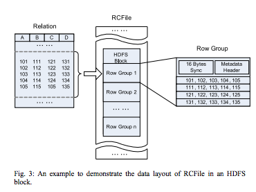
RC File

I have been wondering how RC file actually works so I took a look at paper.
followings are simple review of paper.

In general, for map/reduce based data warehouse, following requirement needs to be addressed.

Requirement

1. fast loading: able to load large amount data fast.

2. fast query process: query execution should run fast.

3. efficient storage space utilization: 

4. strong adaptivity to highly dynamic workload patterns: 

To achieve above requirement, there have been 3 major data placement scheme.

1. row-store

cons

• can`t provide fast query execution(full scan on all records, no skip on unnecessary columns)
• can`t get high storage space utilization since it is hard to compress row efficiently

 pros

• fast data load
• strong adaptive ability to dynamo 

2. column-store

cons

• tuple reconstruction cost lots => query processing slow down
• record reconstruction overhead => since record reside on multiple location in cluster, network cost goes high.
• require pre-knowledge of possible queries for creating column groups

pros

• at query execution time, can avoid reading unnecessary columns.
• high compression ratio

3. PAX store

cons

pros

What RC File provide

1. horizontally partition rows into multiple row groups

2. column-wise data compression within row group + lazy decompression during query execution

3. flexible row group size, trade off data compression performance query between execution performance

4. guarantees that data in the same row are located in the same node

5. column-wise data compression and skip unnecessary column reads

row group in RC File

1. sync marker: at beginning of the row group

2. metadata header: for row group: # records, each column bytes, each field in each column bytes.

3. table data section: column-store, columnA`s fields, columnB`s field….. sorted order

4. RLE for metadata header

5. each column is compressed independently using heavy-weight Gzip => lazy decompression

future work: automatically select best compression algorithm for each column according to it`s data type and data distribution

TODO: take a look at org.apache.hadoop.hive.ql.io.RCFile and others

Belief Propagation for music recommendations with Mapreudce And Giraph

I am taking Probabilistic Graphical Models course from Coursera. once class covers inference on markov random field using label propagation, I wanted to see how this algorithm works on real data so applied label propagation on million song dataset to feel it.

here is example of label propagation.

simple arithmetic result to following.

50% from my profile + 40% from X +10% from Z = 60% rock, 40% jazz.

Generalization

Here is actual formulation. here markov random field is represented by factor graph.

Above formulation can be implemented by matrix multiplication using Map/Reduce.

definition

Lets say graph structure as G, and set of Concept C = {c1, c2,...} where each ci is consist of set of vertices in G. ci represent prior per concept i. then we want to calculate pair-wise posterior given G, C.

implementation

iteration 0: CV(|C| x |V|) x G(|V| x |V|) = CV'(|C| x |V|)
iteration 1: CV'(|C| x |V|) x G(|V| x |V|) = CV''(|C| x |V|)
..
..

each iteration is simply matrix multiplication between Concept-Vertices CV matrix and static graph structure G.

This operation quickly becomes huge. so I first implemented this as DistributedRowMatrix in Mahout.

DistributedRowMatrix class provide following APIs.
1. tranpose: this.tranpose()
2. times(DistributedRowMatrix other): this.transpose().times(other)

using above API, label propagation in Map/Reduce becomes following.

1. init Concept-Vertices matrix CV.
2. normalize Graph for convenience if G is not normalized.
3. create CV, G using DistributedRowMatrix class.
4. for # iteration CV = CV x G

Following code demonstrate how DistributedRowMatrix in mahout library becomes handy.

1:    DistributedRowMatrix CV =   
2:    createInitialCV(numItems, getTempPath("initial.class"),   
3:                    getConf());  
4:    for (int i = startIteration; i < iterations; i++) {  
5:     log.info("current iteration: {}", iteration);  
6:     /*  
7:       GNorm is DistributedRowMatrix   
8:       contain vertex-vertex graph structure.  
9:       DistributedRowMatrix.times calculate  
10:      this.transpose().times(other). so transpose itself first.  
11:      */  
12:     CV = CV.transpose().times(GNorm)  
13:    }  

Note that using Map/Reduce for iterative job is inefficient, so why not try Giraph?

in Graph-Parallel environment, problems become following.

1. each vertex has it`s neighbor edges in G.
2. at superstep 0, some vertex has C vector as value([ci:prior, cj:prior...]). if vertex has C vector, then send C to all of it`s neighbors otherwise don`t send it.
3. after superstep 0, all vertex get messages([vertex_id j, C vector]) from each of it`s neighbors.
if current vertex is Vi, and message is [Vj, Cvj] then edge(Vi, Vj) / Vi`s all Edge sum * C is added to Vi`s value Cvi vector. merge all concept-prior vectors sent to each vertex and update value(Cvi).
4. if iteration is not done, send value(Cvi) to all neighbors.

Following code is compute method in VertexProgram to implement above.

@Override  
  public void compute(Iterable<MultiLabelVectorWritable> messages) throws IOException {  
   /*  
    * each vertex has Vector as value.   
    * this Vector consist of [concept_id:probability,....]  
    * MultiLabelVectorWritable to represent   
    * (vertex j which sent this message, vertex j`s value Vector)   
    */  
   long step = getSuperstep();  
   if (step < iteration) {  
    // we still need to compute on this vertex.  
    Vector currentVector = getValue().get();  
    // create new messages from this vertex.  
    MultiLabelVectorWritable newMessage = new MultiLabelVectorWritable();  
    // set message source to this vertex.  
    newMessage.setLabels(new int[]{(int)getId().get()});  
    // vertex value vector [concept_id:probability] is sparse.  
    Vector newMessageVector = new RandomAccessSparseVector(minNonConceptVertexId);  
    // iterate messages sent to this vertex and merge them up to build this vertex`s vector.  
    for (MultiLabelVectorWritable message : messages) {  
     int messageId = message.getLabels()[0];  
     Vector conceptProbs = message.getVector();  
     float weight = getEdgeValue(new LongWritable(messageId)).get();  
     Iterator<Vector.Element> probs = conceptProbs.iterateNonZero();  
     while (probs.hasNext()) {  
      Vector.Element prob = probs.next();  
      int conceptId = prob.index();  
      currentVector.set(conceptId, prob.get() * weight);  
     }  
    }  
    // prunning for absorb  
    Iterator<Vector.Element> iter = currentVector.iterateNonZero();  
    while (iter.hasNext()) {  
     Vector.Element e = iter.next();  
     if (e.get() < gamma) {  
      continue;  
     }  
     newMessageVector.setQuick(e.index(), e.get());  
    }  
    newMessage.setVector(newMessageVector);  
    sendMessageToAllEdges(newMessage);  
   } else {  
    voteToHalt();  
   }  
  }  

I implemented demo using label propagation with open dataset from million song dataset challenge from Kaggle. This demo load taste profile graph data into memory and calculate on the fly rather than using Giraph for demonstration. here is github for Giraph/Mahout code and demo codes.

TODO: since test set for this data is opend(competition is over), I will measure truncated mean average precision to evaluation label propagation.

movie recommendation demo with matrix factorization

I was experimenting with Graphlab and Mahout for Matrix Factorization these days.

Matrix factorization transform both items and users to the same latent factor space so they can be compared directly.

Even though Mahout and Graphlab is great tool for matrix factorization, these are designed for batch process. to get recommendations for new users who rate existing movies in rate matrix, following two steps are necessary.

1) transform user-rating vector to user-latent feature vector.
2) compare all movie-latent feature vectors with 1) and calculate scores.

this demo ask user to rate movies and do 1), 2) step.

most of work is just glue codes from Mahout with Jetty. 

check out this and feel free to give me any feedback.

Update: added label propagation to find serendipities. since the training data is small enough(1.7 million user, 40 K movies,  19 million edge), just load training data into memory.

Todo: I will update with evaluation metric(RMSE, MAP, Precision-Recall) after running batch jobs for this dataset using mahout/Graphlab for ALS, Giraph for label propagation.

also, add item-based cf as baseline to compare result

Mapreduce, BSP and Graphlab

개인적인 관심사가 machine learning인지라 평소에 주로 map/reduce를 사용한 mahout을 이용해 필요한 알고리즘들을 사용하곤 했다.  요사이 매달리고 있는 matrix factorization문제를 해결 하려고 시도하다가 알게 된 점 들을 몇자 적어본다. 

mahout을 너무너무 잘 쓰고는 있지만 몇가지 map/reduce model의 근본적인 문제를 계속 마주치게 되는데, 첫 째로 iterative job처리가 inefficient하다는 것이다. 

Iterative job을 map/reduce로 구현 할 때의 문제를 좀더 자세히 들여다보면 아래와 같다.

위 그림에서 눈여겨 볼 inefficient 한 곳은 두 가지 이다.

1. 하나의 iteration내에서도 처리해야 할 데이터가 특정 CPU(computing resource)으로 몰려서 partition될 경우 다른 CPU들은 기다리는 lagging이 발생한다. 실제로 사용자 log graph들은 많은 수의 edge를 가지는 몇개의 vertex들을 가지는 경우가 흔하고, 이런 vertex들이 bottle neck 으로 작용한다.
2. 매 iteration마다 발생하는 barrier부분에 disk IO와 startup cost가 있다. map only job이 # iteration만큼 hdfs에서 input을 읽고, 결과를 hdfs에 쓰는 overhead가 있다.

이를 그림으로 표현 하면 아래와 같다.

이러한 iterative한 job을 효율적으로 처리하기 위해 나온 것들이 구글의 pregel이고 이와 비슷한  framework로 apache Giraph, Hama가 있다(꼭 iterative job만을 위한건 아님, 뒤에 설명). 

이중에서 사용해 본 Giraph로 간략히 설명을 하면(자세한 설명), map only잡을 한번 submit하고, map only job에서 여러벌의 worker와 master를 생성한다. 이 master는 각각의  worker에 partition ownership을 부여하고, vertices를 partitioning한다. 

각각의 worker는 자신에게 속한 vertices들에대해 compute를 하고 barrier에서  sync한다(iteration횟수만큼 반복). 

map/reduce와 달리 hadoop의 startup penalty를 한번으로 줄이고, 각각의 superstep(iteration)의 결과들을 hdfs가아닌 memory에 들고 있어 다음 superstep에서 훨씬 빠른 access가 가능하다.

둘째로  interdependent computation(graph-parallel algorithm)은 not map-reducible하다.

조금더 일반화 하자면 많은 수의 machine learning algorithm들은 다음과 같은 property를 갖는다.

현재 vertex  X3의 computing을 위해서 X3의 neighbor들의 value들이 필요한 경우가 많은데 이는 mapper끼리 통신이 불가능한 map/reduce model에서는 처리 하기 힘들다.

label propagation algorithm(graph-parallel algorithm)을 예로 그 일반적인 특성을 보자.

실제로 belief propagation같은 algorithm은 mahout의 DistributedRowMatrix를 이용하여 matrix로 바꿔서 생각하면 구현 자체는 쉽게 할 수 있다. 하지만 matrix형태로 생각하는 게 intuitive하지도 않고, 위에서 말한 첫번째 이유에 의해서도 map/reduce말고 다른 computing model을 찾게 된다.

여기서 이 포스트의 주인공인 Graphlab이 등장하게 된다.

위에서와 같이 machine learning algorithm을 data-parallel과 graph-parallel로 구분 했을 때 Graphlab은 Graph-parallel algorithm에 특화된 framework이다.

살짝 중간 정리를 하자면, map/reduce가 key, value pair에 map/reduce라는 computation을 정의 하는 framework였다면 Graphlab은 graph상의 vertex node에 gatter, apply, scatter라는 computation을 정의 하는 framework이다.

이 framework에서는 각각의 vertex는 사용자가 정의 한 vertex-program을 통해 필요한 computing을 하는데 이때 neighbor vertex들의 상태값 뿐만아니라 다른 vertex의 상태 값들도 mpi를 통해 얻어 오는 api가 제공 된다.

다른 말로 위에서 말한 sparse data dependencies는 graph를 통해, local updates는 vertex-program를 통해 만족된다.

이는 사실 위에서 언급한 Pregel(Giraph, Hama)과 거의 흡사하다. 차이점이라면 pregel은 각각의 vertex-program이 message를 통해 interact하고, Graphlab은 각각의 program이 dependencies가 있는 서로의 state를 access할 수 있다는 점이다.

무슨 소리인가? 아래를 보자.

여기서 가장 중요한 점은 asynchronously이다. 위에서 설명 했던 BSP model와의 가장 큰 차이점은 바로 이 asynchronous한 execution이다. Graphlab은 이런 asynchronous update를 scheduling하면서 consistency를 보장해 주는데, 이를 위해 아래와 같이 scope rule이라는 개념을 가진다.

결론적으로 vertex consisitency가 가장 parallel하고, full consistency가 가장 non-parallel하다. 알고리즘 별로 어떤 scope rule이 필요한지 정의하면 framework이 race condition과 deadlock이 발생하지 않도록 보장해준다.

version1(shared memory)에서는 데이터가 커지면 memory도 커져야 했었지만, version 2부터는 distributed version으로 이런 제약이 없어졌고, HDFS를 input/output으로도 사용할 수 있게 되었다. 또 매우 다양한 algorithm들을 toolkit으로 제공하고 있어서 당장 사용해 볼 수 있다는 장점도 있다. 

자세한 내용은 http://graphlab.org/에서 꼭 살펴보길 바란다. 

http://videolectures.net/nipsworkshops2010_guestrin_kml/는 SELECT lab에서 NIPS2010에 발표한 video이다. 

reference:

http://graphlab.org/

TODO: 

1. Graphlab과 mahout을 benchmark 해본 결과 정리
2. MPI + Graphlab setup tutorial
3. Giraph 자세한 설명 페이지 정리

running median problem

I found this interesting problem from interview street.

problem was to maintain running median from stream of numbers.

more formally,  following is full problem from interview street.

The median of M numbers is defined as the middle number after sorting them in order, if M is odd or the average number of the middle 2 numbers (again after sorting) if M is even. You have an empty number list at first. Then you can add or remove some number from the list. For each add or remove operation, output the median of numbers in the list.

Example : For a set of m = 5 numbers, { 9, 2, 8, 4, 1 } the median is the third number in sorted set { 1, 2, 4, 8, 9 } which is 4. Similarly for set of m = 4, { 5, 2, 10, 4 }, the median is the average of second and the third element in the sorted set { 2, 4, 5, 10 } which is (4+5)/2 = 4.5  

Constraints:

0 < n <= 100,000

1. naive

If n is small enough, problem is simple.

each insert/delete sort entire elements

this require n * nlogn(n operation x cost for sorting).

2. using two multiset

Thing is only few elements are affected when insert/delete operation happen.

solution using two multiset s1, s2.

invariant

1) s1 is supposed to maintain 0 ~ n/2th order statistic.

2) s2 is supposed to maintain n/2 ~ nth order statistic.

3) s1.size()  and s2.size() only differ at most 1.

to hold invariant 1, 2

we compare x(current value to insert or delete) with maximum of s1 and minimum of s2 to decide where to put x.

to hold invariant 3

we need re-balance step

this can be done in constant time by

1) moving minimum of s2 to s1

2) moving maximum of s1 to s

Solution

once 3 invariant is meet, then calculating median as problem description is trivial.

1) s1.size == s2.size(s1.size + s2.size is even), then return (maximum of s1 + minimum of s2) / 2.0

one tip we should take care of integer overflow when we average two value(32bit integer) since adding two 32bit integer can cause integer overflow.

2) otherwise if s1.size > s2.size, return maximum of s1. s1.size < s2.size, return minimum of s2.

finally checking if we can delete x is trivial, since multiset provide find method in O(logN) complexity.

just good enough pass testcases.

3. using skip list

I was wondering what about more generic cases.

few google search gives me link to skip list.

for this problem, we exactly need indexable skip list since we keep need to extract median as input comes.

obviously this problem can be solved by indexable skip list.

here is my simple implementation.

TODO

want to take a look at how redis use skip list and understand why skip list is better than self-balance-tree in distributed environment.

check out code here

ALS-WR

Alternating-Least-Squares with Weighted-lambda-Regularization(ALS-WR)

Purpose

ALS-WR 는 model-based 방식으로 원래 matrix R을 iterate하면서 U, M 두개의 matrix로 factorize한다.

R = (user, item, rate)형식의 matrix로 U X I의 사이즈를 가진다.

원래는 R안에 대부분의 R(i, j)는 다 비어 있다. Collaborative Filtering의 목적은 이 비어 있는 R(i,j)들을 어텋게 예측 할 거 인가이다.

Background

CF는 크게 3가지로 나뉜다.

방식	장점	단점
memory-based	결과이해 쉬움, 구현 쉬움, centent frer	사람이 매기는 rating에 섞인 noise에 대처 미흡, spare한 data에선 performance down, new user/new item에 no result, not very scalable.
model-based	rate자체보다는 training set의 pattern이용, sparse data에 비교적 강함, 직관적 결과이해	model building에 비용 큼, scalability 와 performance간의 trade off, reduction model때문에 원래 useful data can be lost
hybrid	memory-based + model-based	비용큼

Introduction

참고:개념이해

논문

시작하기 전에 matrix factorization에 대한 설명(?정확히는 svd개념설명)으로 링크를 달아 놓았다.

ALS-WR는 model-based방식으로써 원래 rating matrix R(user x item)을 least squared error 를 최소로 하는 U(user x hidden feature), M(item x hidden feature)로 factorize하는 알고리즘이다.

말은 거창한데, 결국 어떤 cost function F(U, M) = square error part + regularization part 을 최소로 하는 U, M을 찾는 문제이다.

자세한 식은 논문을 참조 하고, 이해한 대로만 의견을 추가하겠다.

앞에 square error part는 (실제 rate R(i, j) - 예측 rate R^(i, j))를 error라고 정의하고, 이 error^2들의 합을 의미한다.

Regularization은 machine learning 분야에서 자주 사용 되는 용어로써, model이 overfit하는 것을 방지하는데 도움을 주는 방식이다.

overfit이 모냐

위의 식에서 전체 cost는 각각의 data들과 예측 곡선 y = ax + b와의 거리들의 제곱의 합이다. 그럼 위의 optimization problem에서 cost 를 최소화 하려면 1차식이 아닌 y = ax^50 + bx^49.... 식의 높은 차원식(곡선이 될것이다?) 을 사용하면 될것이다. 문제는 굉장히 복잡한 식을 써서 training set에서의 cost를 최소로 만들어 봐야 training set을 잘 대변 할 수 있지는 않다. training set을 잘 대변 하는 식을 찾아야 test set에서도 잘 작동하는데, training에 특화된 높은 차원식은 보통 test set에서는 높은 error를 보인다. 이를 이 높은 차수의 식은 overfit되었다고 한다.

다시 말해 cost를 최소로 하는 U, M을 찾는것이 문제이고, 이때 overfit을 방지하기 위해 regularization part를 추가 한 것이다.

algorithm(아주간략)

ALS-WR는 M을 고정하고, U를 optimize하고, U를 고정하고 M을 optimize하는 일을 한 번의 iteration으로 한다.

처음 M은 평균 rating들에서 작은 random number만큼의 차이가 나는 임의의 rate로 initialize되고 iteration을 거치면서 M과 U를 optimize한다.

Recommendation

결국 최종적으로 R^(i, j)를 어텋게 예측 하느냐는 다음과 같다.

ALS-WR를 통해서 R => U, M으로 factorize된다. 다른말로 U는 user를 hidden feature space로, M은 item을 hidden feature space로 project하여 hidden feature space에서의 similarity를 측정하여

user의 item에 예상 R^(i, j)를 계산 하게 된다.

R' = U x transpose(M)이 된다.

Test

mahout-0.6-snapshot을 이용하여 test 해보았다. Cluster는 8 core, 16G서버 10대

Iteration #	Hidden Feature #	RMSE	Running time
20	30	0.9167081037790646	2 hour